Jan 10 2026 The most important sorting algorithm (that you can memorize)

Algorithms: a personal story

In the past, I've always thought of algorithms as my soft spot in my programming arsenal. Unlike many of my colleagues who started learning programming from solving algorithm problems and took prizes in programming competitions, I started learning programming at a young age just to try making computer games. So I was exposed to a lot of pragmatic programming early on (like making games and apps with GameMaker and Lua), but didn't know how to implement a linked list for quite some time.

Later after I switched my major to Computer Science, I was pretty bored out of my Algorithms class. Our professor was just reciting things from the titular CLRS textbook line-by-line. I did learn a few important concepts like invariants and big-O notation and dynamic programming 1 - but the actual algorithmic details were just alien to me. I really didn't get how the inner workings of a red-black tree would actually help me in programming novel things, when in practice you would just use the standard library in your choice of language. So these algorithmic details were just content to temporarily memorize in order to get good grades, and I soon forgot most of it.

Even during my undergraduate years, I was still into making computer games. Although a lot of that was with using the Unity engine, I was also interested in creating my own engine with C++. That naturally led me to studying computer graphics, and now I was hammering OpenGL code to render stuff on the screen. And in order to achieve a smooth 60 FPS real-time without lag, the algorithms started to be visible in my eyes and actually had consequences. (Also, unlike the algorithms in CLRS I actually needed to care about the underlying hardware details!) So came spatial partitioning structures, along with various kinds of geometry-related computations. Later on during grad school where I worked on researching topics on computer animation, I naturally became interested in implementing physics engines, which required a whole bunch of new techniques in order to crunch numerical computations as much as possible in real-time. Which is where I've discovered (or re-discovered) counting sort, the first algorithm that I was actually able to fully memorize by heart, and which also changed my way of programming things permanently.

Enough of the tangents, let's get straight into the algorithm!

Counting sort

Let's say you have a list of integers, and you want to sort them. The textbook answer for the algorithmic complexity is (for a comparison sort). If you don't have any more assumptions about how the data is distributed, then this is the best you can get.

But sometimes you actually have a list of integers of a limited range, and often there are many repeating elements. For example, a list of random integers from 0 to 4:

[0, 3, 1, 2, 4, 2, 1, 1, 0]

Which we want to sort as:

[0, 0, 1, 1, 1, 2, 2, 3, 4]

Is there a way to do this in linear time, instead of ? Let's formulate the problem properly: Given an array of size of integers in the range ~ (where M is typically much smaller than N), can we sort it in ?

Here's counting sort in all its glory (written in a C-like syntax 3). If you compress the code it's only about 10 lines:

int N = ...; // Input array count
int M = ...; // The range of integers [0, M)
int arr[N] = {...}; // Input array

int sorted[N]; // Output array

int starts[M+1] = {0}; // temporary buffer for our algorithm, cleared to zero before usage

// Pass 1 (Forward pass): Increment count
for (int i = 0; i < N; i++) {
    int item = arr[i];
    starts[item] += 1;
}

// Pass 2 (Prefix sum)
for (int i = 0; i < M; i++) {
    starts[i + 1] += starts[i];
}

// Pass 3 (Backward pass): Decrement count and insert
for (int i = N - 1; i >= 0; i--) {
    int item = arr[i];
    starts[item] -= 1;
    sorted[starts[item]] = item;
}

You just need to remember that there are three for loops, each of them having a distinct purpose.

1. The first pass scans through the input array and counts the occurrences for each category (by "category" I mean the range of integers ~ ), and stores it in the starts array. (In more elegant terms, we call this a histogram) For our little example, the starts array becomes:

// Category:       0   1   2   3   4
starts =          [2,  3,  2,  1,  1,  0]

You might have several questions:

• Why is this temporary array called the "starts" array?
• Why is there an extra empty slot at the end?

Don't worry, all of this will become clear later on!

2. The second pass does something we call a "prefix sum" on the starts array we created earlier - we sequentially increment the next count with the previous count to create an increasing list of integers:

// Category:      0   1   2   3   4
// starts[i]      2   3   2   1   1   0
// starts[i+1]       +2  +3  +2  +1  +1
starts =         [2,  5,  7,  8,  9,  9]

Notice that we also populate the final slot. This has a purpose later on, keep on reading!

3. Now here is how the "starts" array becomes important: We use this as bookkeeping for where we want to insert each item into the output array, determined by category. For each item, we retrieve the appropriate starting index from the "starts" array, decrement that by one, and use that as the index to insert into the output (sorted) array. When you finish iterating the array backwards 2, the starts array now starts at zero, and the resulting output becomes:

// Category:      0  1  2  3  4
starts =         [0, 2, 5, 7, 8, 9]
sorted =         [0, 0, 1, 1, 1, 2, 2, 3, 4]

If you are cunning enough - you might be able to now understand what the starts array means. If you cannot see it, I'll add some spaces for a hint:

// Category:      0     1        2     3  4
starts =         [0,    2,       5,    7, 8, 9]
sorted =         [0, 0, 1, 1, 1, 2, 2, 3, 4]

When there are many duplicates in your array, your sorting result will have "clumps" of elements grouped together. And the starts array precisely tells you how these elements are grouped together. So although this array was initially just a temporary array needed for sorting, it turns out that it actually tells you more about the distribution of your sorted data, so don't throw it away! We're later going to see how we can use this to our advantage.

It's all about the Data Structures, not the Algorithms!

So far we've only sorted integers - but the real power of counting sort is in how it can organize various types of data in an efficient manner. Let's look at a more realistic example! Now we have a list of more OOP-like generic objects with a "category" or an enum tag, that can be represented as a limited range of integers.

struct Item {
    string name;
    string description;
    Category category;
}

Our task is to group elements with the same value, which is typically called the "Group-By" operation. This is one of the most frequently used operations to organize data! 4

The naive freshman-like way to do this is to use a hash table, since hash tables can insert / retrieve anything in O(1) (at least, in theory):

unordered_map<Category, vector<Item>> groups;

for (auto& category : ALL_CATEGORIES) {
    groups[category] = vector<Item>();
}

for (auto& item : list) {
    groups[item.category].push_back(item);
}

But hash tables are much more detrimental to performance than you might think. Even if you use open addressing, there is a lot of bookkeeping involved in maintaining a hash table, and the nature of hashing forces you to do lots of random memory accesses which can destroy your performance if used in the wrong way (at least, if the category size is large enough)!

A much better way to store the groups is to map each category to an integer starting from 0 to 25, and storing as an array instead:

vector<vector<Item>> groups;

Which is better, but still there's lots of indirection: we're storing a nested list so the memory for the items will be scattered throughout memory, and cache locality will suffer. 5 A much better way to store the items would be to use a flattened array:

vector<Item> sorted;

...but then how are we actually going to know which entity is in which group? Remember the starts array from earlier? We can see that they contain the starting index for each category, assuming that the list of items is sorted! Let's tweak the counting sort algorithm to obtain a sorted list of items, as well as calculating the start buffer (two birds with one stone)!

for (int i = 0; i < N; i++) {
    Item item = arr[i];
    starts[item.category] += 1;
}

for (int i = 0; i < M; i++) {
    starts[i + 1] += starts[i];
}

for (int i = N - 1; i >= 0; i--) {
    Item item = arr[i];
    starts[item.category] -= 1;
    sorted[starts[item.category]] = item;
}

After obtaining the sorted array and the starts array, we can easily retrieve the items per each category like:

void print_items_in_category(Category category) {
    int start_idx = starts[category];
    int end_idx = starts[category + 1];
    for (int i = start_idx; i < end_idx; i++) {
        println(sorted[i].name);
    }
}

Note that we need that extra slot in the starts array (which contains the item count) in order to obtain the end index! Without this, the code would be more complicated because of the edge-case handling (and it's easy to miss this out-of-bounds error):

int end_idx = category == (NUM_CATEGORIES - 1)? items.size() : starts[category + 1];

You can also retrieve the number of items in each category as:

int count = starts[category + 1] - starts[category];

So you don't actually need to store a separate counts array to store the item counts for each category, it's just two (consecutive) array accesses and a subtraction. Feel free to wrap these operations inside OOP-like methods. You can use spans/iterators/generators to return the list without allocating additional arrays, depending on the language you use. For example in C++ (or other similar languages):

class GroupedItems {
    vector<Item> sorted;
    vector<int> starts;

    span<Item> get_items_in_category(Category category) {
        Item* item_start = sorted.data() + starts[category];
        int item_count = starts[category + 1] - starts[category];
        return span<Item>(item_start, item_count);
    }
}

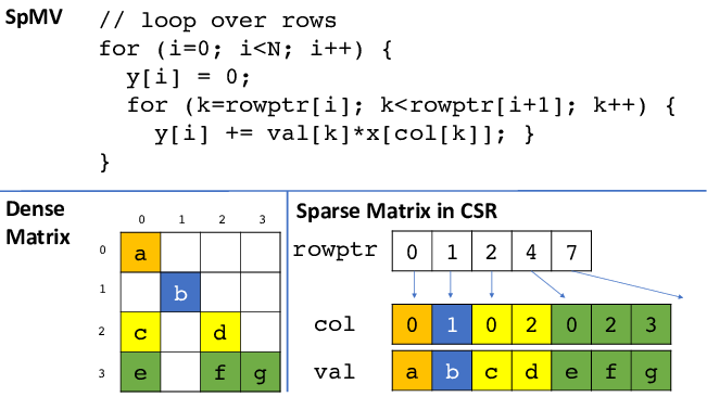
By the way, if you have any background in numerical computation... this is also how a sparse matrix is usually implemented - the Compressed Sparse Row (CSR) format! In CSR, you store non-zero values row-by-row in a flat val array, and a rowptr array tells you where each row starts - exactly like our starts array. So that means if you want to build a sparse matrix structure from a different data structure (ex. list of (row, col, value) entries), you can just do counting sort on it and voila, you get the exact data structure you want.

The most flexible sorting algorithm

The best part of counting sort is that it's actually really easy to memorize - and you can customize to your liking whenever you need it. There is little value in creating your own counting_sort() function in your utility library and trying to make it reusable 6 - since the real value in this algorithm lies in being able to take it out of your head at any time line-by-line and wield it as some sort of magical weapon, whenever you're in a scenario where performance is of utmost importance.

Let's say that the tags are not stored in the object, but need to be computed via the get_category() function (which runs fast). Then you can just compute the categories inside the counting sort loop, and the algorithm becomes:

for (int i = 0; i < N; i++) {
    Item item = arr[i];
    starts[get_category(item)] += 1;
}

for (int i = 0; i < M; i++) {
    starts[i + 1] += starts[i];
}

for (int i = N - 1; i >= 0; i--) {
    Item item = arr[i];
    int category = get_category(item);
    starts[category] -= 1;
    sorted[starts[category]] = item;
}

You do have to run get_category() twice, once during the forward pass and the other during the backward pass. However, if the mapping function is cheap enough, then it actually makes sense to run it twice, rather than allocating an extra "categories" array to store and re-use the information. 7 You frequently have to do trade-offs between computation and memory allocation / access when you're writing efficient data-oriented algorithms, and counting sort makes this trade-off very easy to implement and experiment with.

What if you just want the names of each item as the sorted output? Then you modify the backward pass:

for (int i = N - 1; i >= 0; i--) {
    Item item = arr[i];
    int category = get_category(item);
    starts[category] -= 1;
    sorted[starts[category]] = item.name;
}

What if you actually have multiple categories per item? (In this case, it's less about the sorting and more about the group-by operation) 8 No problem-O, modify the forward and backward passes:

for (int i = 0; i < N; i++) {
    Item item = arr[i];
    for (auto& category : item.categories) {
        starts[category] += 1;
    }
}

for (int i = 0; i < M; i++) {
    starts[i + 1] += starts[i];
}

for (int i = N - 1; i >= 0; i--) {
    Item item = arr[i];
    for (auto& category : item.categories) {
        starts[category] -= 1;
        sorted[starts[category]] = item;
    }
}

All of these modifications make the algorithm flexible enough that you're going to use the least amount of computation and memory allocations/accesses for a given problem. For example, if you were just using a generic sorting algorithm (like std::sort if you're using C++), you might have needed a second pass to convert a list of items to a list of names. But in here, this is fully embedded inside the sorting process, so computation is done as efficiently as possible.

Lastly, what if your integer range is too big? In this case, you can divide your integer range into digits, and then run a counting sort for each digit starting from the least significant digit. And congratulations... you've invented radix sort, where the complexity is instead of 9! (This is actually taught in most Data Structures or Algorithms classes, but counting sort is only mentioned as sort of an implementation detail and not an important algorithm in itself. What a bummer!)

Verdict

The reason why I like the counting sort algorithm is that it's really simple to implement, yet flexible enough to adapt to whatever problem you're solving. For a summary:

1. When your keys are bounded integers, you can sort your data in linear time.
2. The starts array isn't just used for bookkeeping, it stores useful metadata about your sorted data!
3. By writing counting sort yourself, you can fuse it with whatever data transformation you need, making it extremely flexible.

You do have to know that it isn't perfect though:

• When M (category count) is large relative to N (item count), and the keys are quite unique / random - either you should use radix sort, or just one of the various assortments of comparison-based algorithms.
• When you need an in-place sort (if your data is really big, and you don't want to duplicate them for a sorting pass).

This was the first algorithm I could recall line-by-line without checking a reference, and once I had it memorized, I started seeing opportunities to apply it everywhere. Before, my mindset was to reach for std::sort (or an equivalent in the standard library), but now I first ask whether I can restructure this as a counting sort problem, and often the answer is yes! Ultimately this is a good lesson on data-oriented design (DOD) - performance is naturally gained from how well you understand your data transformation problems.

1.

^ Mostly from Eric Demaine (MIT Open Courseware), his Youtube videos are god-tier. I think Eric Demaine is kind of like Jesus sent from God for students who have to deal with a crappy Algorithm lecture and have to self-study that goddamn book.

2.

^ You don't necessarily need to run the last for loop backwards - in fact the algorithm runs perfectly if you run it in the original order. However, doing the pass backwards ensures that the sorting is stable (in other words, the order between duplicate elements in the original array is respected in the sorted output). Which can be quite nifty in many cases, so keep that in mind!

3.

^

Note that pass 3 can be more succinctly expressed using C's unary decrement operator as:

int item = arr[i];
sorted[--starts[item]] = item;

But I've refrained from using it since not everyone enjoys the obtuse dark arts of C.

4.

^ It's the GROUPBY operation in SQL! C#'s LINQ also has the GroupBy function, though I'm not sure if it's implemented with counting sort.

5.

^ This is assuming that you're using a value-oriented language such as C++, Rust, Go (or C#, if you use structs), where you can actually have control over how your objects are laid out in memory. For languages such as Java, JS/TS, Python, etc. you're often forced to have boxed objects in the GC heap anyway, so you do not have control over these details most of the time.

6.

^ Since I have mostly used C++ during my career, I have tried implementing a fancy templated version of counting sort where you can pass in InputMapper and OutputMapper as lambda functions - but to be honest the complexity wasn't worth it that much. I've learned over the years in general to not be too afraid of having repeats of similarly-looking code, when you're doing performance-sensitive stuff!

7.

^ This technique is the basis of matrix-free methods (a technique for solving linear equations quickly in a parallel fashion, especially on the GPU). Inside the algorithm you compute the same values multiple times, which seems unnecessary but it's actually justified because you don't need additional memory to load/store intermediate values from/to global memory all the time.

8.

^ This actually comes up a lot in computer graphics. Let's say we have a polygonal mesh, with each face having a list of vertices or edges. If you want to find the reverse mapping (a list of adjacent faces per each vertex) - a typical grad-student quality code would involve haphazardly creating a hash table, But guess what - counting sort can come to the rescue and eliminate all your memory allocation woes in your mesh processing code.

9.

^ Technically where = digits and = radix.